DIY Magnetometer for Geophysical Survey and Archaeology

What is under the ground? What is under my property? I have studied geography, I have an old house that has been standing as a farm for over a hundred years on a wide piece of land and I like to work with Arduino & Co. So I build my own magnetometer.

With a magnetometer you can map archaeological structures that cause anomalies in the Earth’s magnetic field. They work best in large open areas and are (hopefully) sensitive enough to pick up the slight changes in the earth’s magnetic field over a particular spot. Magnetometer mapping can reveal patterns by recording the magnetic properties of ferrous elements in the soil or those left behind after human activity.

The idea is to plot the magnetometer data on a map, visualise differences and therefore get an insight into the underground.

For example, magnetometry was used in the exploration of the ground around Stonehenge in England. However, they have better sensors there and drag them across the field with a quad. But hey, my device costs less than 50 Euros.

Two years ago I already walked over my property with a single magnetometer sensor, recorded GPS data and magnetic values and transferred them to a custom Google Maps map. The result was interesting, but not very meaningful. For more data, I would have had to walk a lot more in a more dense grid.

So how about seven sensors side by side? Do I then need 7 GPS receivers? No, I can calculate the position of the sensors starting from the center coordinate if I have a compass that shows the current direction.

It is not my intention to find expensive treasures. But knowledge is also a treasure.

Supplies

Arduino Mega 2560 (has enough analog pins)

7 Hall sensors ("49E 011BD", 10 for ~9 Euros)

GPS NEO 6M

Compass LSM303

OLED 1.3"

SD card reader

Cables

Plastic rail (or wood) and plastic screws

2 wheels, metal spindle, wood

Arduino IDE https://www.arduino.cc/en/software

qGIS (Freeware) (https://www.qgis.org/en/site/forusers/download.html)

Step 1: Planning

Magnetometers are used in archaeology and geography to "see" beneath the earth's surface. The magnetic field of our earth can be easily detected with a compass whose needle always points north. But with a sensor, you can measure the strength of this magnetism much more precisely. For our device, we don't need to calibrate our sensors to a certain value, because we don't need absolute measurements but only want to detect the relative differences over a relatively small area.

Step 2: Scheme

The Arduino should collect some data for us; GPS-position, seven magnetometer values, compass heading and calclulation of new coordinates for each sensor. Then it should write the values to the SD card, which we then transfer to a map.

Step 3: Calculations

Since I do not want to use a separate GPS device for each sensor, the remaining coordinates are calculated. Of course, I don't always want to have to go strictly north. Sensors 1-3 and 5-7 rotate around sensor 4/GPS. I use a digital compass to determine the direction of travel.

The zero point of our local coordinate system is the origin coordinate (our GPS device), D is the distance of the desired sensor from the GPS device, e.g. 0.25m. We first calculate in the unit metre, with the help of the formulas:

Longitude: ((cos(compassheading) * distance) *conversionFactorX);

Latitude: ((sin(compassheading) * distance) *conversionFactorY);

With *conversionFactor we convert the metres into decimal places of the coordinates:

The distance of the longitudes decreases, starting from the equator, at the poles the lines even meet.

At the equator, the earth has a circumference of 40075.017 km. Divided by 360°, this gives a distance of 111319.49166m between the lines of longitude. Multiplied by the cosine of the current latitude (about 48° for me), we get the actual distance in metres.

float conversionFactorX = (1/(cos(lat)*111319.491666666));

The latitudes have the same distance from each other everywhere. The distance pole-equator is divided by 90°, which results in:

10,007.555km/90° = 111.195055555 km per 1°.

Therefore, the following is given in the Arduino-sketch:

~~conversionFactorY = (1/111195.0555555)~~

Because the Arduino could not calculate well with the number and gave wrong decimal places, I had to write the factor as a power of ten:

float conversionFactorY = 8.993205633*10E-6;

Depending on which quadrant of our local coordinate system the sensor is located in, the coordinate distances are added or subtracted from the original GPS coordinate.

In the Arduino sketch it looks like this for example:

lon5 = lon + ((cos(heading) * distance)*conversionFactorX);

lat5 = lat - ((sin(heading) * distance)*conversionFactorY);

Step 4: Construction of the Arduino Device

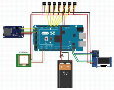
The power supply runs for all devices via 5V and Gnd

Data connections:

Hall sensors: A1-A7
GPS: 18 (TX1), 19 (RX1)
Compass: SCL, SDA
OLED: SCL, SDA (next to USB plug)
SD card: CS 53, SCK 52, MOSI 51 , MISO 50

For other Arduino types (e.g. Arduino Nano) the connections and the software must be adapted accordingly.

First I tried out all the connected devices separately. Later, I combined the connections and software and coordinated them with each other. At first with the help of a breadboard. When the cables became too confusing, I built a plug-in board for the Arduino Mega and soldered the necessary connections. This way I can fit the device into a housing better and without loose contacts.

Step 5: Software

Download 'field-magnetometer.ino' and load it onto your Arduino.

During operation, the device writes a csv file to the SD card. This data can either be loaded into a GoogleMaps map, GoogleEarth pro or the software qGIS to create maps. (Step10: qGIS and maps)

field_magnetometer.ino (see below)

qGIS (Freeware) (https://www.qgis.org/en/site/forusers/download.html)

Hall-sensor.ino to see sensor values

calibrate_compass.ino for the exact adjustment of the compass

Step 6: Construction of the Sensor Phalanx

The seven Hall sensors are mounted on a plastic rail (or a wooden board) at 25 cm intervals. I use plastic screws for this so that as little metal as possible can falsify the measured values. In addition, hot glue was used.

The middle sensor will later be assigned the coordinates of the GPS receiver. The coordinates for the other measuring points have to be calculated (see Step 3).

For attaching the wires I first used a wire winder. This wraps the cables tightly around the connections. In addition, I fixed the whole thing with heat-shrink tubes.

The sensors are connected in parallel to the power supply. A data line goes from each sensor to the micro-controller. For convenience, I have built a plug with which I can connect an extension cable between the phalanx and the device.

Step 7: Construction of the Trolley

Of course, you can also carry the instrument and sensors. But it is more comfortable with a trolley.

The cart can be built individually from existing materials. I used the axis and wheels of an old lawn mower. The rest is made of wood.

It was important to me that the handrail is at a height of one metre and that the sensor phalanx can be driven as far as possible in front of me. I used only a few screws and some wooden dowels to avoid possible interference with the sensors by metal.

The wheels have a positive effect: in a meadow, I can easily see where I have already gone by looking at the tyre tracks.

Step 8: Enclosure

I use a 5-euro wooden box from the craft shop as the housing, but you can also use a simple cardboard box. Fit the device into the box and make suitable cut-outs for the display and the connections.

The compass and GPS receiver, which are mounted outside the housing, get their own cover made of old screw boxes or other packaging material. Transparent housings would be good, then you can see when the GPS receiver starts blinking.

Step 9: Data Test

Warm up: After switching on, the GPS device needs a few minutes to receive signals from some satellites. The magnetometer waits for the coordinates even though the GPS is already blinking.

Attention:

A stationary GPS receiver strangely records large jumps in coordinates; with a moving receiver, the coordinates are stable. For example, when I am sitting in my office, recording GPS data and later viewing it on a map, I "jump" back and forth up to 50 meters. (The nicest jump I recorded was from Germany to 150 kilometres west of Paris.)

The first tests I did with the not-yet-finished device. You can see my walk through the garden with only one sensor.

The second try with all sensors was more successful.

Next try: The compass is now properly calibrated, therefore the sensors are displayed at right angles to the direction of march. The Hall sensors do now measure the same values at the beginning.

Step 10: QGIS and Maps

Now we still have to visualise our data set. Can we see anything at all?

I first tried Google Maps. It is relatively easy to use, but I was not so happy with the graphical results. Besides, you need a Google account, which not everyone likes.

After some trial and error, I decided on qGIS. It's free and a very nice tool for our purposes.

qGIS:

a) Load data:

First you have to download and install qGIS (Freeware) (https://www.qgis.org/en/site/forusers/download.html)

Layer --> Add Layer --> Add Delimited Text Layer

Get the file, format ".csv"

X Decimal separator is comma

X First record contains field names

X -field longitudes y-field latitudes

Coordinates reference system: EPSG:4326 - WGS 84

"Add" and close this window. The data are loaded.

b) Add a map as a background:

Web QuickMapServices OSM OSM Standard

c) Edit data points:

In the layer window on the left: Klick MAGDATA (or your data file) with right mouse button. -->Properties

in the properties window, at the top select Graded

Value: magnet

Method: colour

Gradient: Set colours as desired

Mode: natural interruptions (you can experiment here!)

Classes: 8 or 16

With "heat map" you can create cloud-like graphics that might show more changes in the underground.

You can also visualise the data in Google Earth Pro (File--> Import -->...). The 3d view is interesting, but the setting options are few.

Step 11: Results

After a few tests, the data is already quite encouraging! I would still have to work with the imaging software.

I am aware that the calculation of the coordinates is inaccurate. Even my small GPS device is certainly not the most accurate on the market. Despite the blurriness of the data, perhaps an approximate image of our underground will be produced and we will get to know our earth a little better.

With the small wheels it's pretty rough on the grass. I am trying to get bigger (plastic) wheels.

Good luck finding your treasure of knowledge!

Step 12: Update

In the last test image, you can see that the magnetometer values in the western test area are clearly different from those in the eastern area. An area of about 350 square metres was surveyed.